Machine Learning on the GPU - Case Study: Open Image Denoise
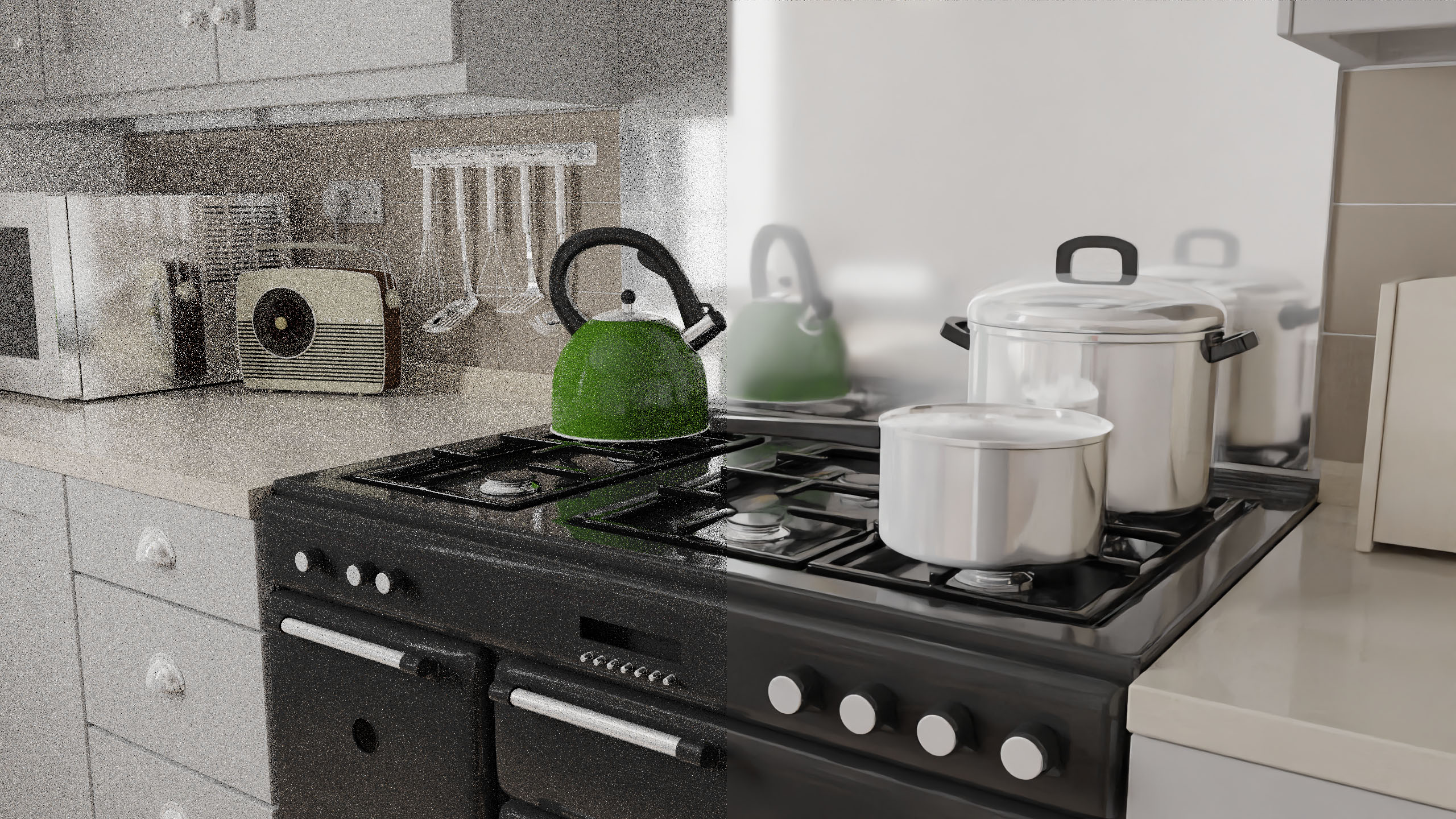
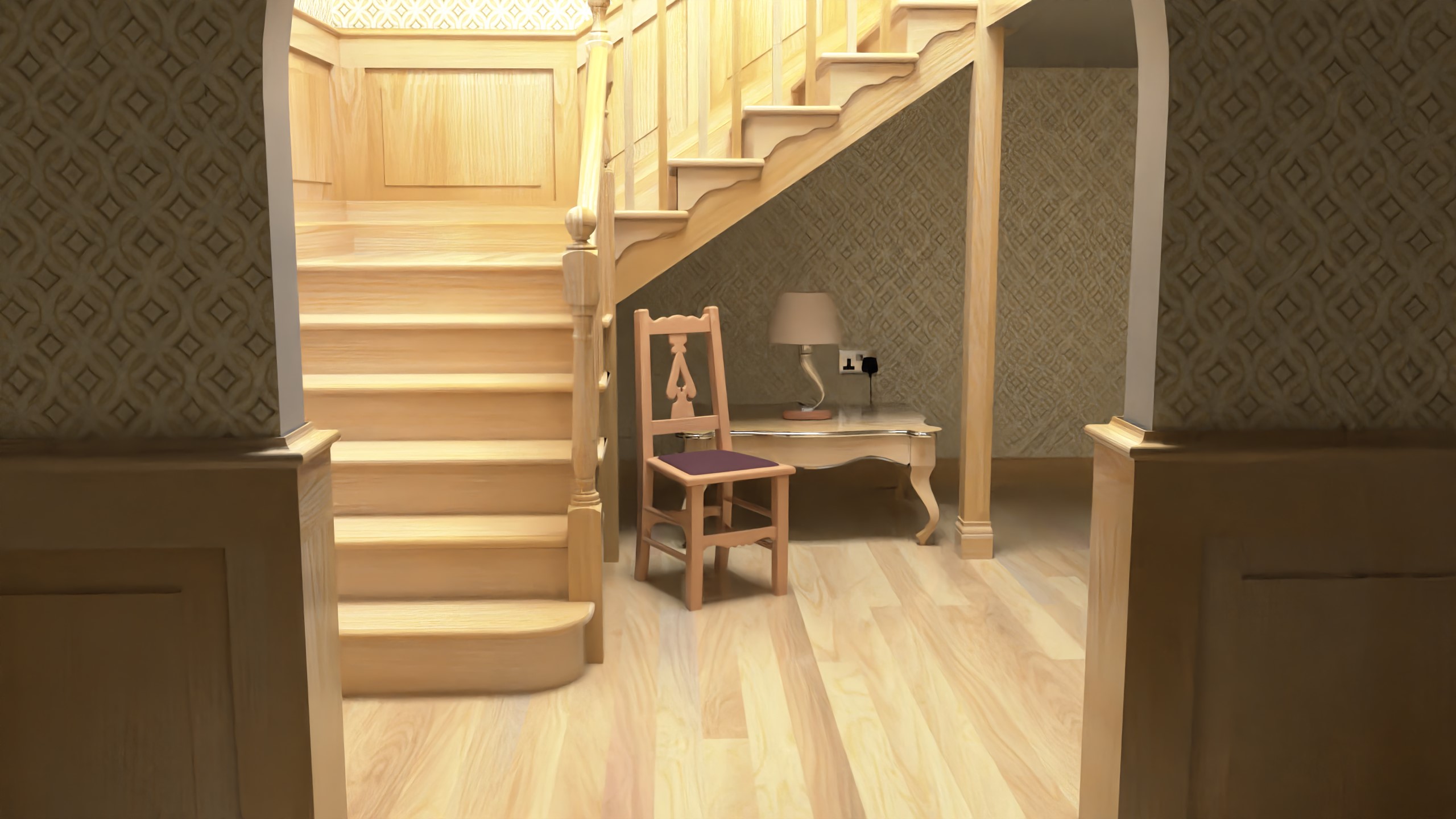
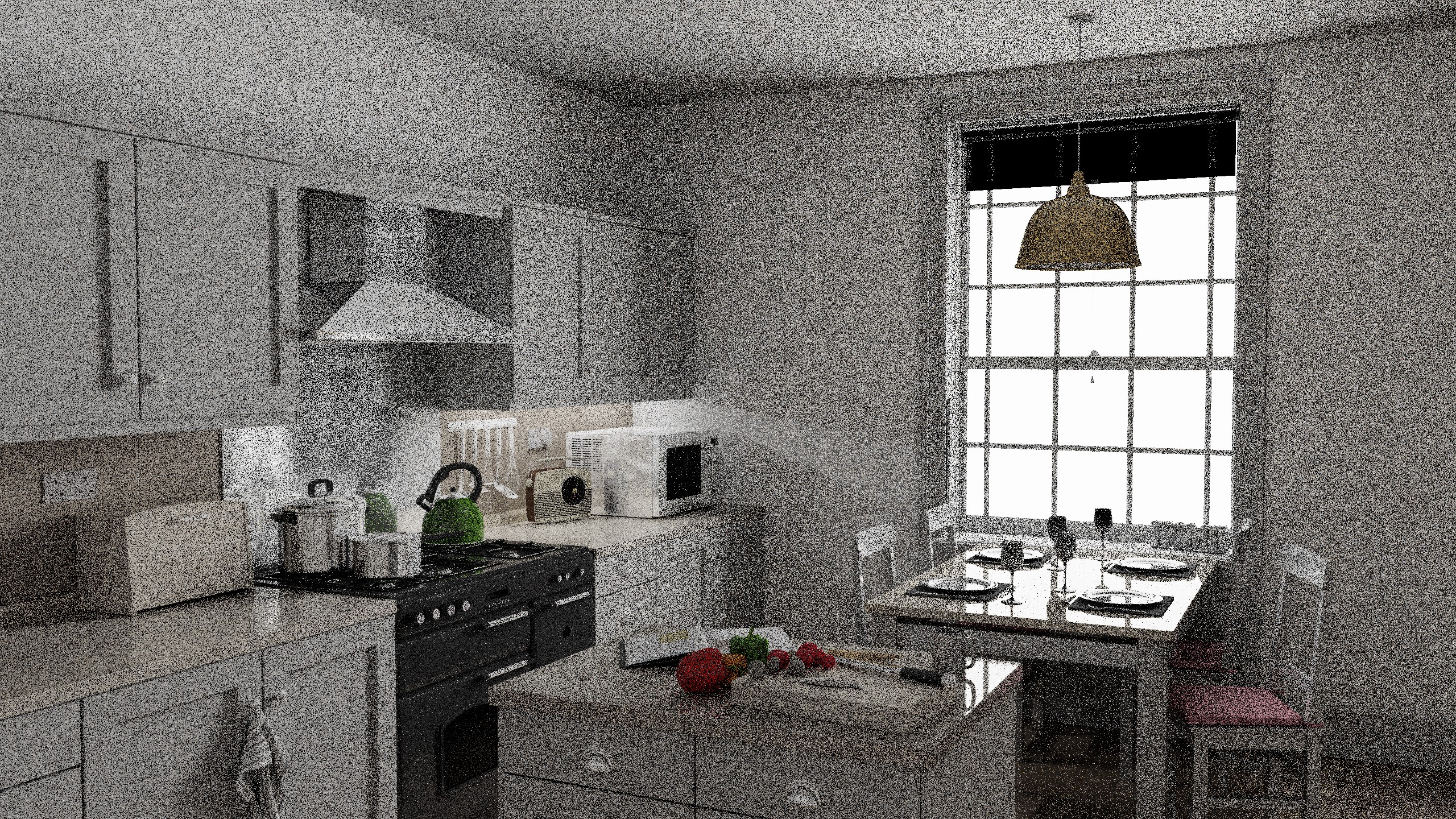
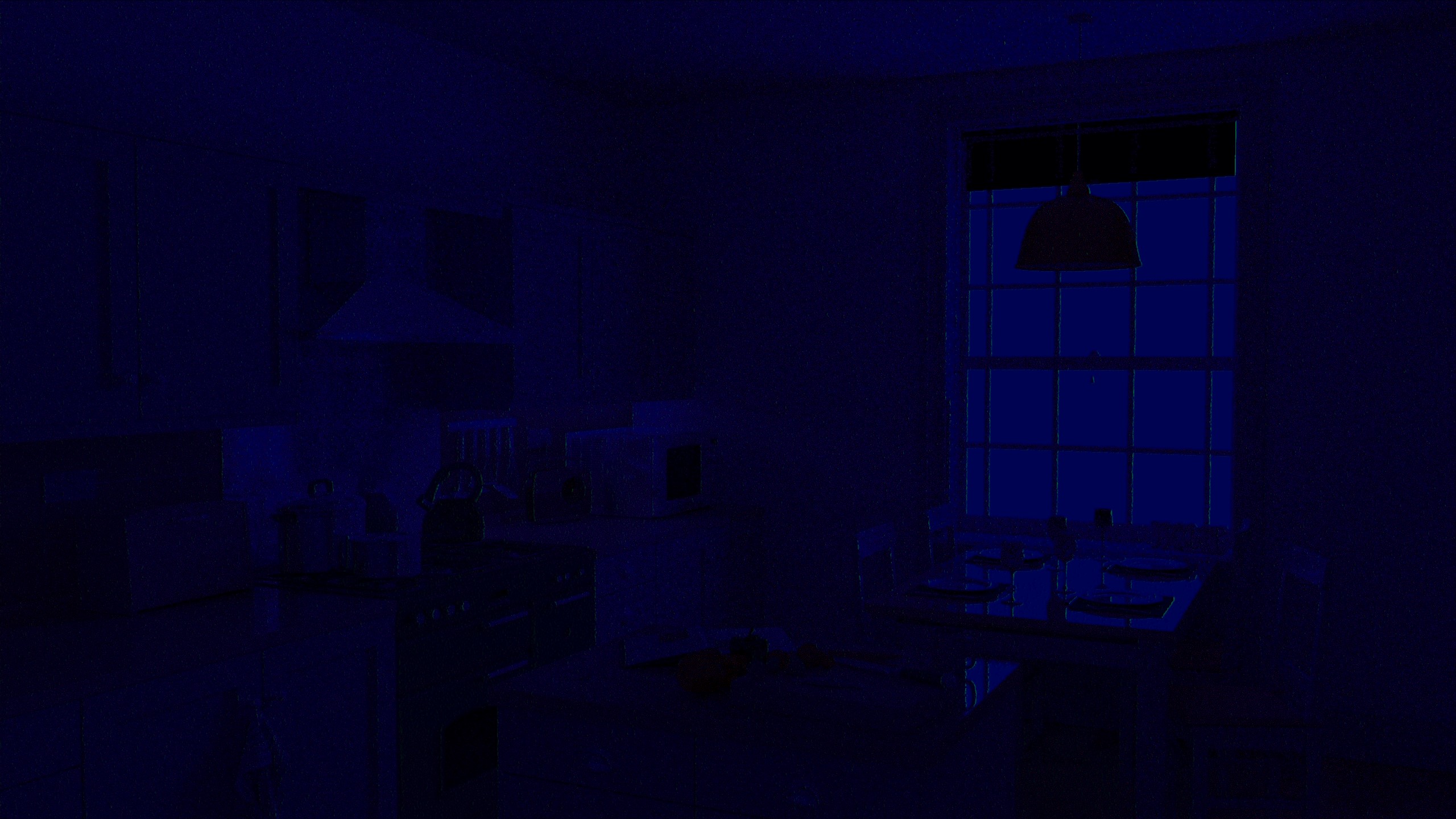
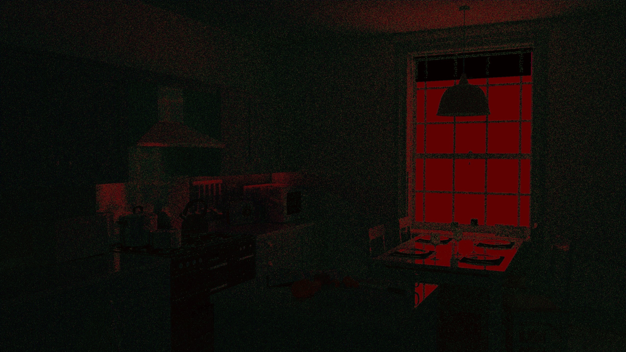
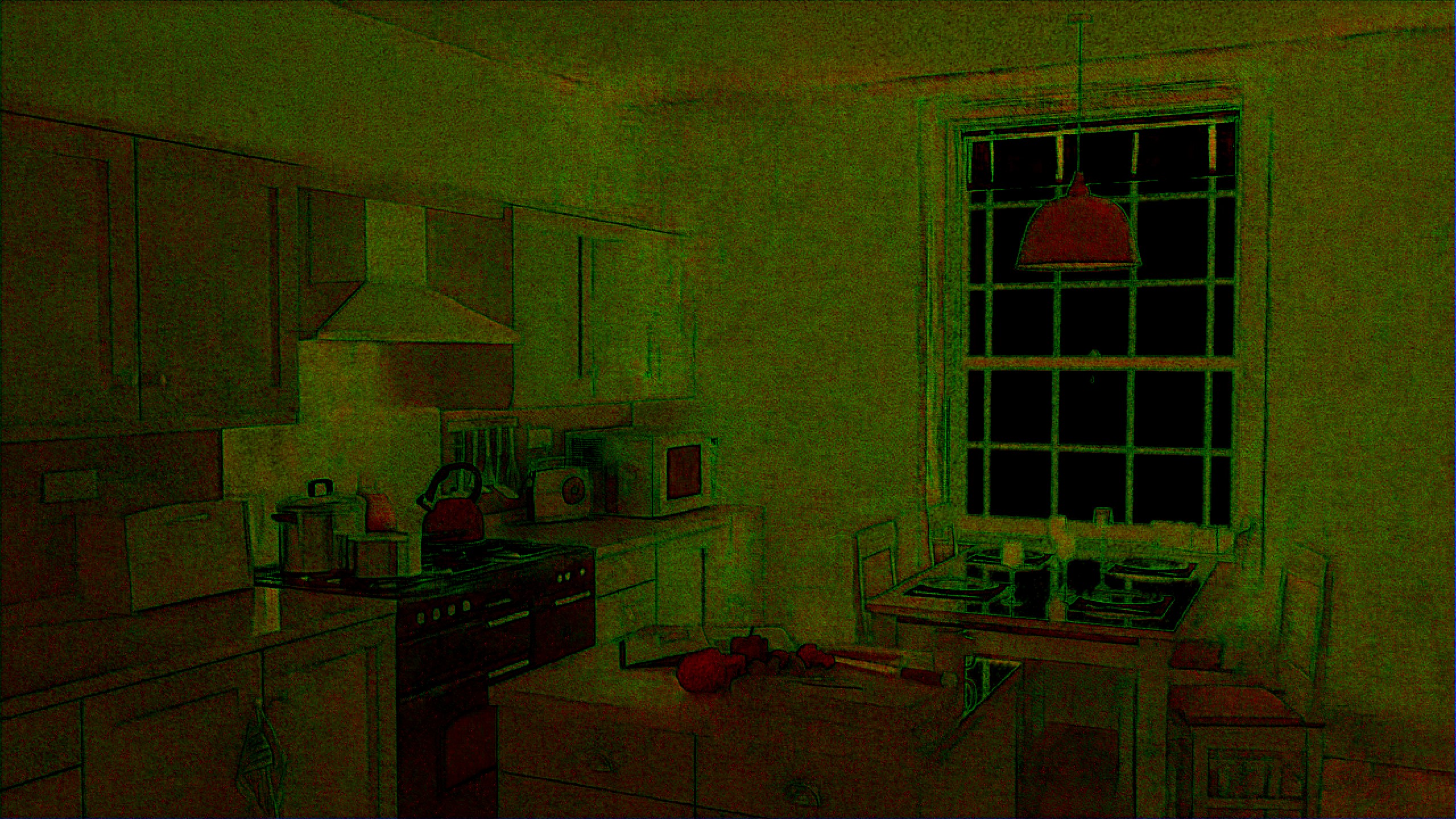
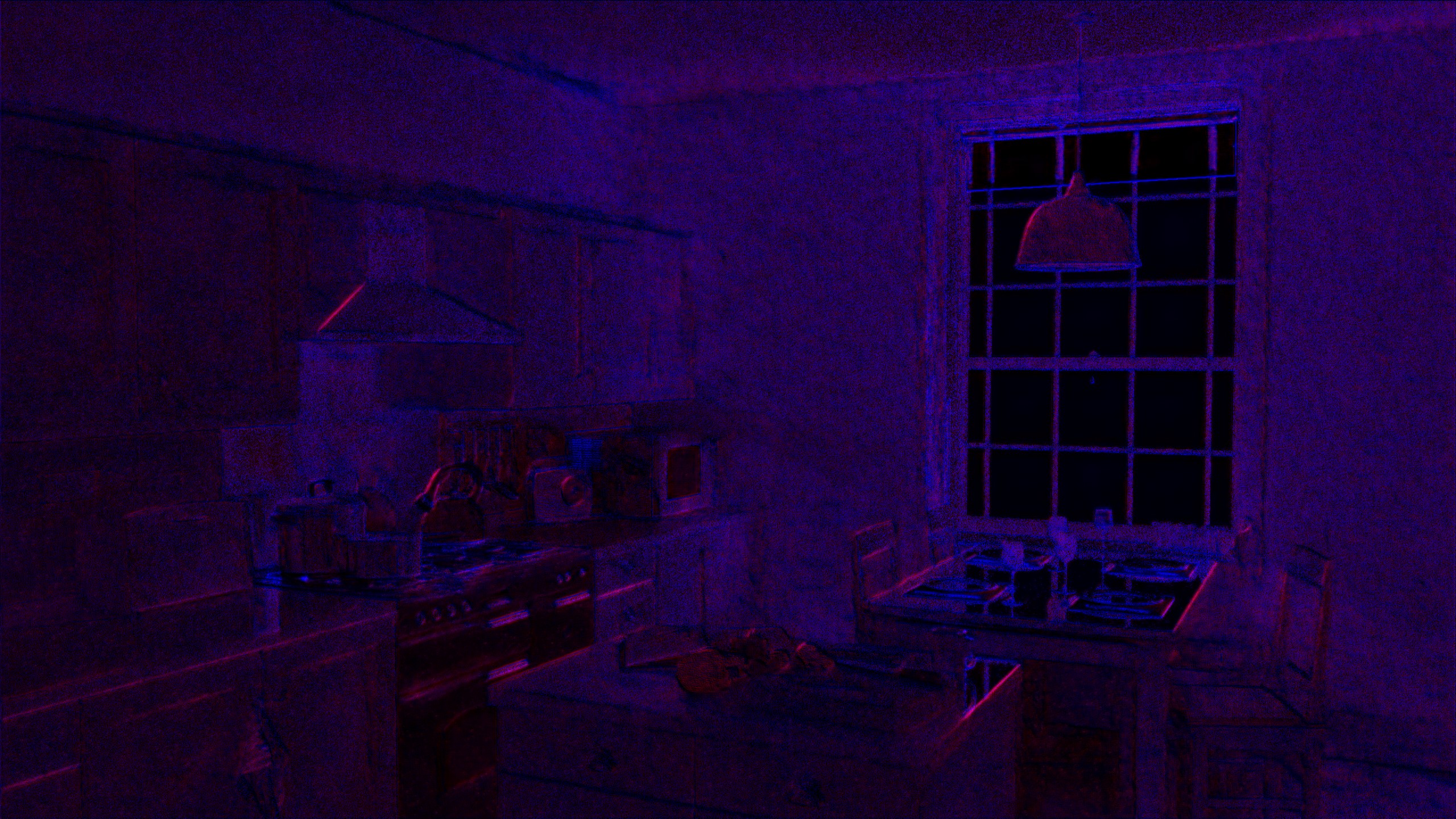
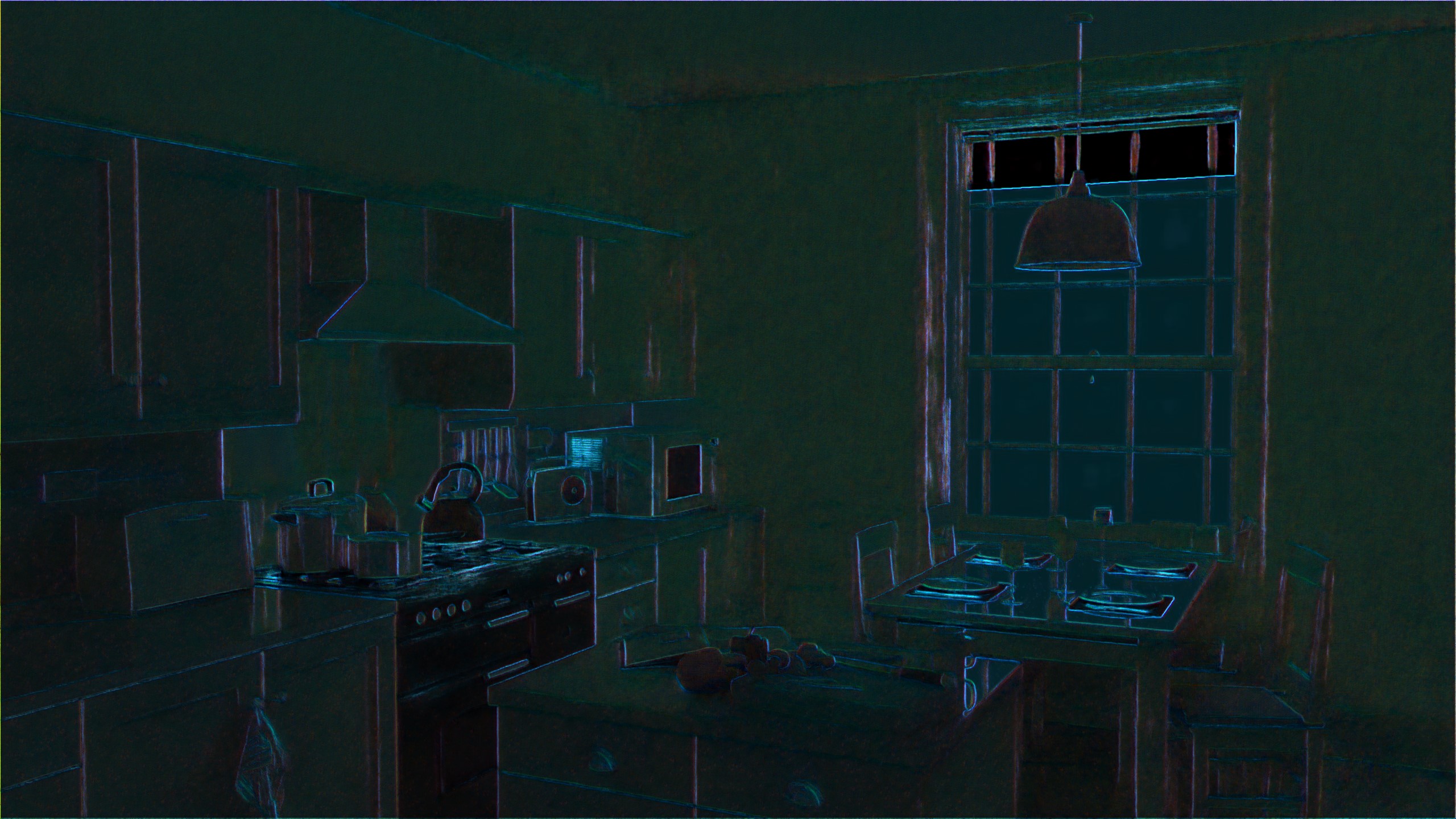
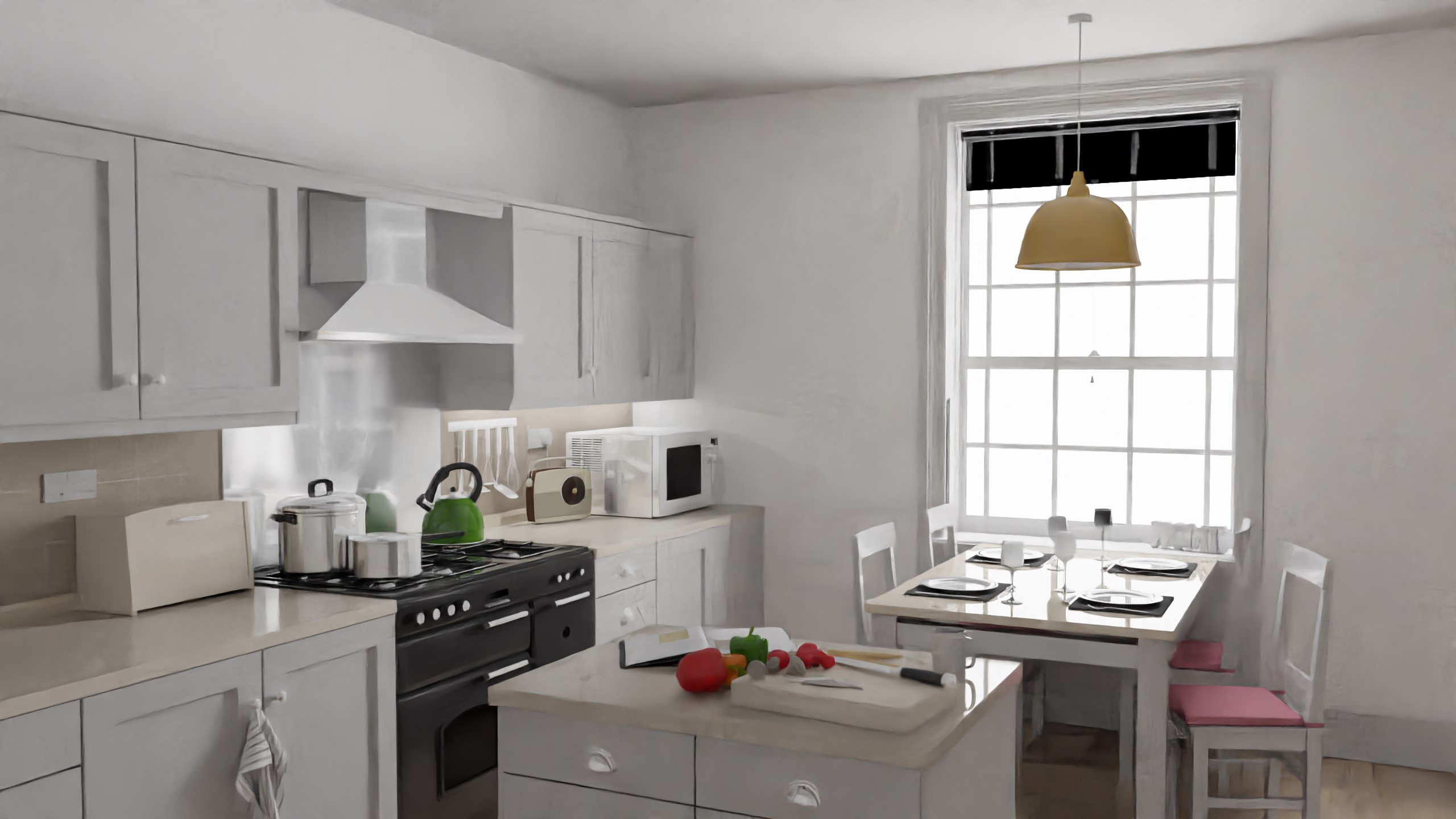
Raw path traced output at 8 samples per pixel on the left and same output but denoised using Machine Learning on the right
Machine Learning (ML) is everywhere! Even on the real-time/gaming side of things, ML is becoming an increasingly important part of the future with already existing techniques like DLSS beating out top non-ML based techniques in visual quality while still being fast enough to run at 60FPS (or even framegen up to 120!). Despite that, most folks even with a deep understanding of how GPUs work, don’t have much of an intuition on what these ML-based GPU workloads are actually doing.
The way I’ve targetted this post is it’s just enough knowledge to make machine learning feel a less like black magic for rendering engineers and begin to develop a vague understanding of of what is actually going on when we talk about tech like DLSS, Open Image Denoise, XeSS, etc. To go about this, I will narrow in on a single case study: Open Image Denoise. I am far from an expert, and in fact I’d consider myself a beginner when it comes to Machine Learning. Almost all of my knowledge stems from some recent work I did to port Open Image Denoise to DirectML in my hobby path tracer.
Let me breakdown those 2 things I just mentioned as they will be a focus in the rest of this post: Open Image Denoise and DirectML:
Open Image Denoise in an open source, ML-based denoiser from Intel that’s used by a lot of the big offline renderers like RenderMan. I’ll refer to Open Image Denoise interchangebly with it’s acroynym OIDN. It is not intended for real-time use in games the way that DLSS or XeSS. That said, it has been optimized to the point that on extremely high-end GPUs, it can be quite fast. This does allow it to be used for quick interactive preview renders. While very little has been disclosed about XeSS/DLSS, we can take some of the inner workings of OIDN and assume some of this does carry over to how those techniques work despite having very different goals.
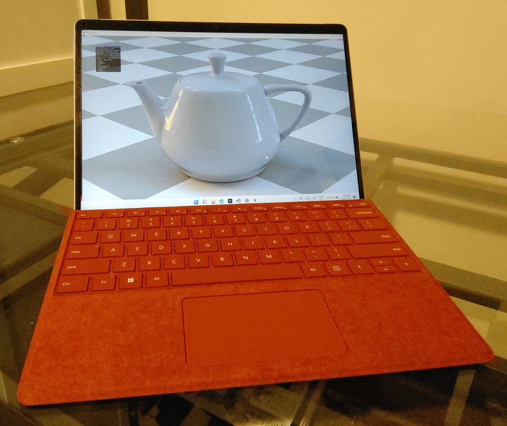
DirectML is the DirectX 12 API for abstracting out machine learning operations, akin to how DirectX Raytracing abstracts the hardware implementation around raytracing. There’s one important distinction here however, DirectML allows these ML operators to run even on hardware that doesn’t have ML hardware acceleration by emulating the operation with a compute shader. This is an important distinction, everything I talk about on this post can be run on basically anything that can read/write from a texture and do some multiplies. That means either the CPU or potato GPUs. In fact, I can even run my DirectML port on my laptop with a 5 year old integrated GPU:
Finally, one last thing before we get into the tech details. We can break machine learning down into 2 big categories: learning and inferencing. This post will only cover inferencing (specfically inferencing on the GPU).
“Learning” is an extremely expensive operation where we feed the ML model loads of input data and try to get it to “learn” to do something. In the case of Open Image Denoise, we feed in a bunch of path traced images with an extremely low sample per pixel (lets say 1-4 rays per pixel) and then also give it matching images with a nearly converged image (imagine >1024 samples per pixel).
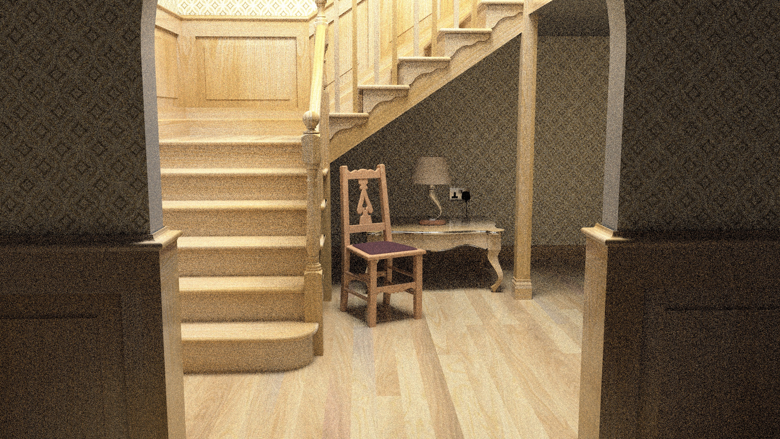
Stairway rendered with 8 spp
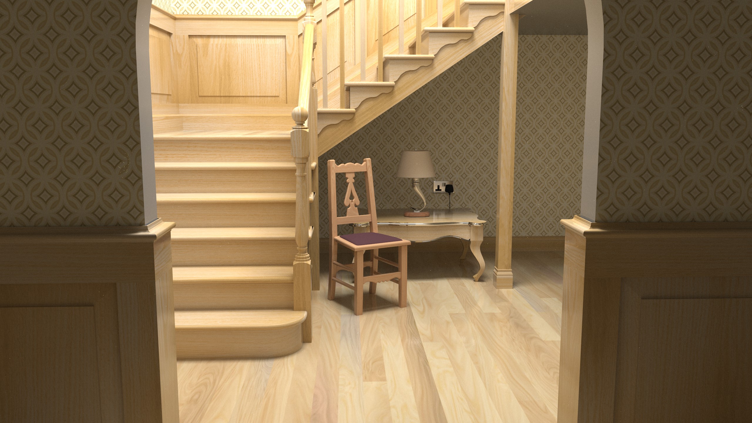
Stairway rendered with 1024 spp
We then ask it to essentially try a bunch of random things to see if it can transform the low sample per pixel images to the converged images. With each attempt it can grade itself by comparing what it output to the converged image. There’s a ton of linear algebra that can help it iteratively learn in a way that’s not just randomly trying things. When it’s done, you’ll get a big list of weights. Later on I’ll talk about how that comes into play.
Now that the learning is done, we can do inferencing, which is MUCH faster and is basically just feeding data in through the model that was created from the “learning” process. Again using Open Image Denoise as an example, we’d feed in a noisy path traced image (likely one it’s never seen before), and it would use it’s learned results to produce a denoised image. This inferencing process is generally what would run on consumer hardware, so optimizing this is important, which is why GPU inferencing comes into play. This process of taking the noisy image and denoising it, that’s what we’re going to dig into.
Stairway rendered with 8 spp but denoised with OIDN
Frame breakdown
Because I’ve ported Open Image Denoise to DirectML, which is just using DX12 under the hood, we can break this down in a way similar to how folks breakdown a frame in video games: GPU capture! I’ve captured a frame in Pix, lets take a look:
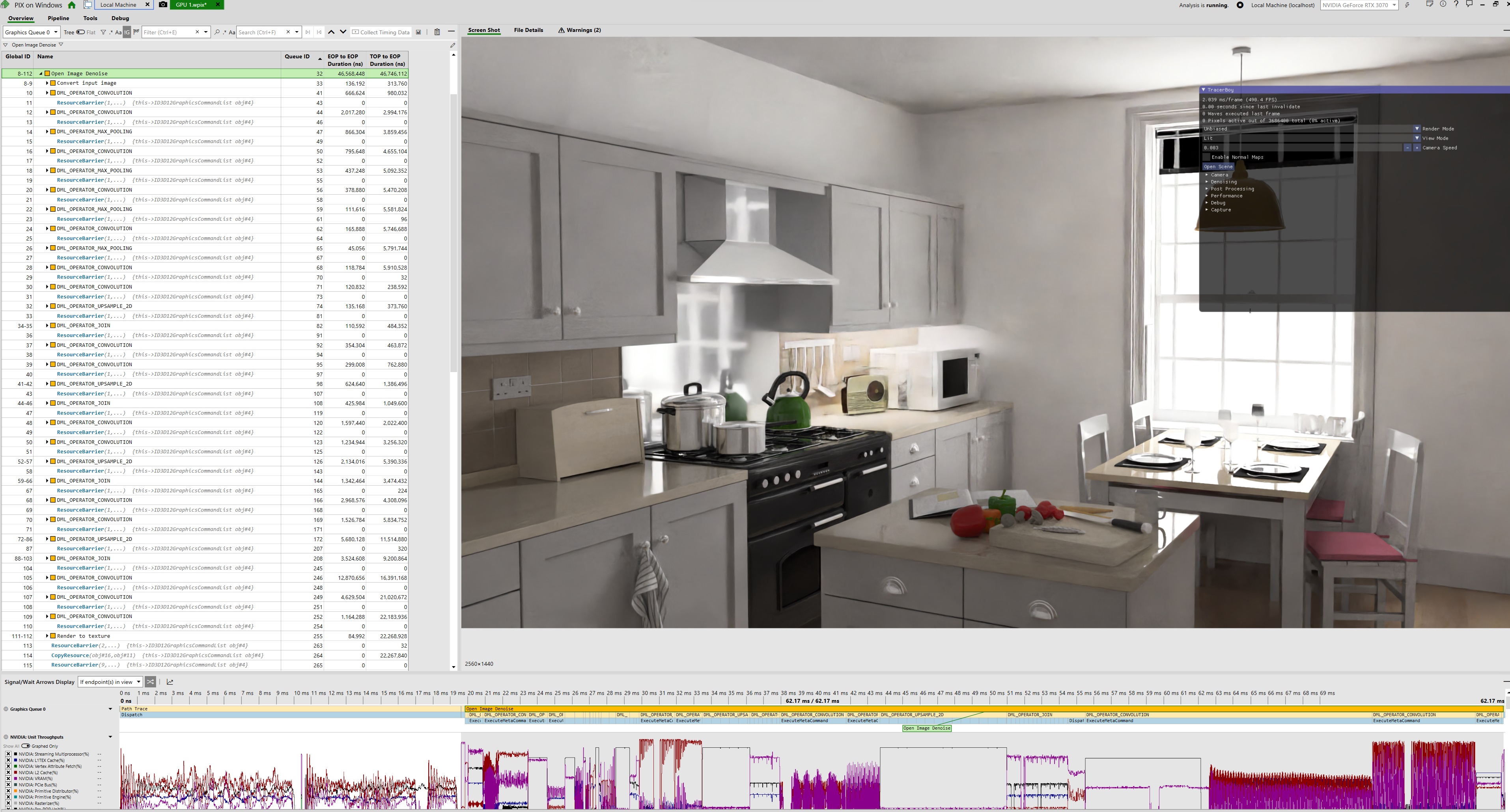
Pix capture of the PBRT kitchen scene ran on an RTX 3070 at 2560x1440
At first glance, there’s a LOT going on here. Most non-ML based denoisers like SVGF would only have around 5-6 operations. And there’s a whole lot of these “DML_OPERATOR” things. But if you take a step back, you’ll notice there’s only 6 unique things happening here:
- Conversion the input inmage to a tensor (and visa versa at the end)
- Convolution Operators
- Pooling Operators
- Join Operators
- Upsample Operators
What I hope to show is that each one of these steps is actually very simple and understandable in terms of what the GPU is doing. Each of these “operators” are actually just compute shaders, and as you’ll see, they’re fairly simple compute shaders. And once you understand all 5 things, you will understand the all the building blocks to a production grade ML denoiser.
Tensors
Lets start with the conversion from render targets to a tensor (and visa-versa). What is a tensor? It’s a broad N-dimensional math thing, but in the context of Open Image Denoise, we can constrain the definition a little bit. Essentially they’re textures that can have an arbitrary number of channels. By default when we think of a texture we’re talking 3 channels: red, green, and blue. However there’s a lot of scenarios in games for example where we might be rendering out a LOT of channels. Lets think something like a G-buffer where we have normals, albedo, roughness, metal, etc. Normally to support this you have 3-4 individual render targets each with 3-4 channels.
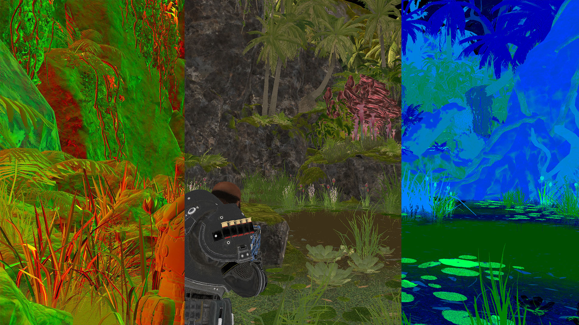
Example of GBuffers from Gears 5: Hivebusters. Left to right: Normals, Albedo, and Material Properties
However imagine you could represent that with a single texture but with 12+ channels. That would be neat! Let me immediately burst your bubble, modern GPUs don’t support anything like this. Why do we care so much about a large channel count? Well, later on we’ll see passes in OIDN that require up to 112 channels in their output. Because there’s no built-in hardware texture format that would allow this, the solution in DirectML is to just linearly represent these textures in a buffer and track the actual channel representation ourselves. We lose the opportunity for HW/drivers to swizzle and arrange channels in a more cache friendly manner but in exchange we get the flexibility of storing as many channels as we want.
And so the resulting compute shader to convert from a 3 channel 2D texture to a tensor is about the most boring shader you can imagine:
Texture2D<float4> inputImage : register(t0);
RWBuffer<half> outputTensor : register(u0);

[numthreads(DIRECTML_THREAD_GROUP_WIDTH, DIRECTML_THREAD_GROUP_HEIGHT, 1)]
void TextureToTensor( uint3 DTid : SV_DispatchThreadID )
{
    if (DTid.x >= Constants.OutputResolution.x || DTid.y >= Constants.OutputResolution.y)
        return;

    uint index = DTid.y * Constants.OutputResolution.x + DTid.x;

    float3 val = inputImage[DTid.xy].xyz;

    outputTensor[index * 3] = val.x;
    outputTensor[index * 3 + 1] = val.y;
    outputTensor[index * 3 + 2] = val.z;
}
I’ve omitted one big topic from the shader, which is different layouts. Because the driver no longer knows about the texture layout, it has lost the ability to intelligently pick how to pack the channels. For example you could pack each channel in it’s own slice or have all channels placed locally next to each other. Depending on many factors, one layout maybe better than the others. You’ll hear terms like NCHW or NHWC which refer to this. Just know that this exists and that they can have a big impact on performance (I saw ~3x difference trying different layouts).
Okay! So we have a rough idea of what tensors are now. Every single operation in DirectML results in a single output tensor that is used as input to the next DirectML operation.
To convert from a tensor to a texture is equally simple. However, I’ve snuck in some extra functionality we’ll find useful here. If we’re converting from a 3 channel tensor, this shader would be just simple as the previous one. And indeed the final output of OIDN will result in a 3 channel tensor that we just need to convert back into a texture. However, we may want to be able to visualize some of the intermediate tensor outputs. And to go further, we may want to be able to visualize different channels in the tensor. To handle that, I’ve added a “SliceToOutput”, that lets you specify which 3 channels to output.
Buffer<half> InputTensor : register(t0);
RWTexture2D<float4> OutputTexture : register(u0);

[numthreads(DIRECTML_THREAD_GROUP_WIDTH, DIRECTML_THREAD_GROUP_HEIGHT, 1)]
void main( uint3 DTid : SV_DispatchThreadID )
{
    if (DTid.x >= Constants.OutputResolution.x || DTid.y >= Constants.OutputResolution.y)
        return;

    // Not handling different size inputs for simplicity
    uint index = DTid.y * Constants.InputResolution.x + DTid.x;
    uint channelOffset = Constants.SliceToOutput * 3;

    float4 color;
    color.r = InputTensor[index * Constants.InputChannelDepth + channelOffset + 0];
    color.g = InputTensor[index * Constants.InputChannelDepth + channelOffset + 1];
    color.b = InputTensor[index * Constants.InputChannelDepth + channelOffset + 2];
    color.a = 1.0f;

    OutputTexture[DTid.xy] = color;
}
Frame Breakdown
Okay now with the background on Tensors out of the way as well as a way to visualize any output tensor in OIDN, we have all the tools we need to visually step through each OIDN operation. Lets take a look:
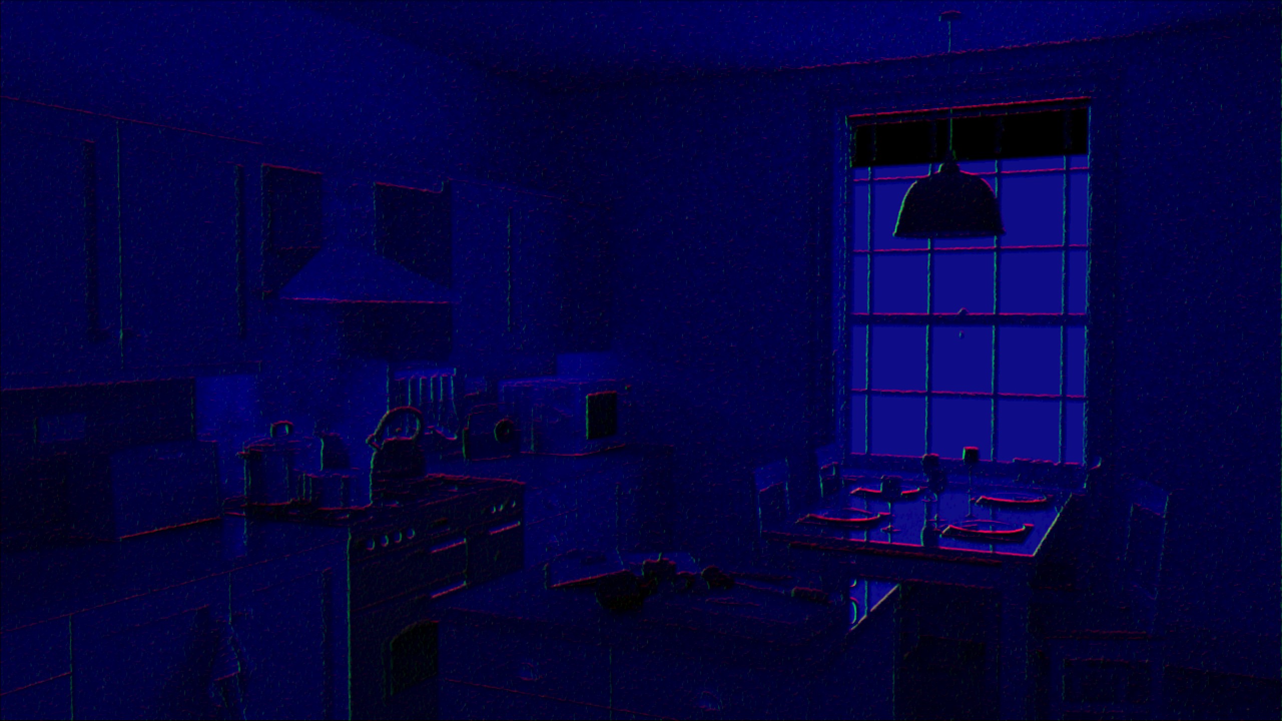
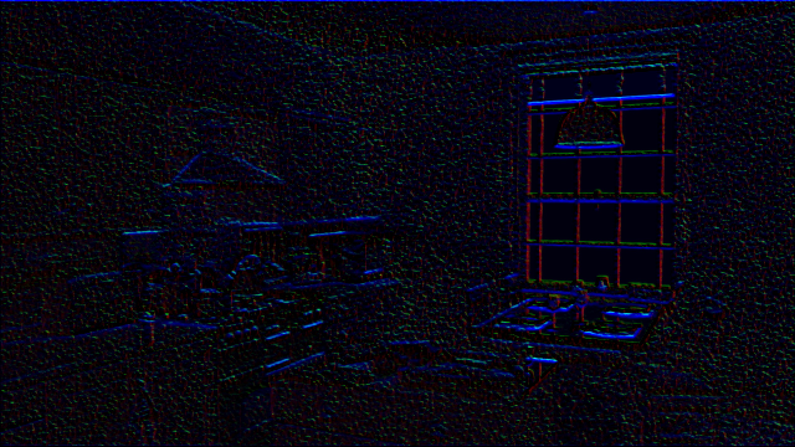
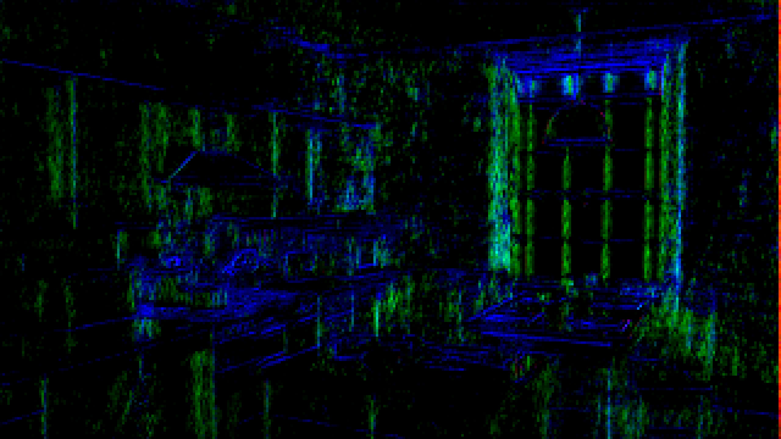
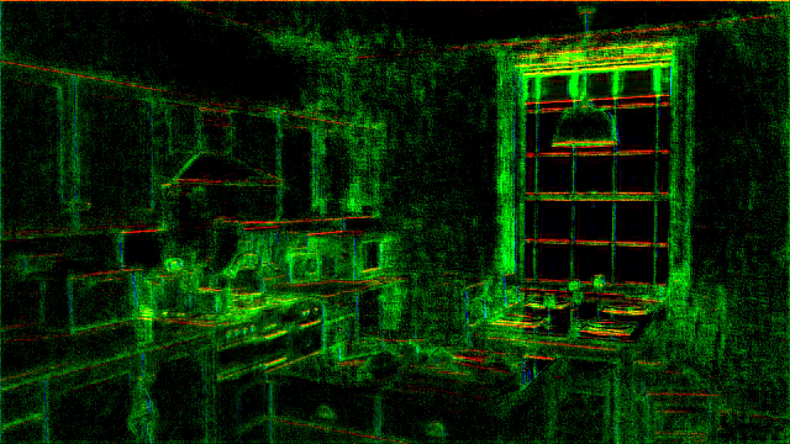
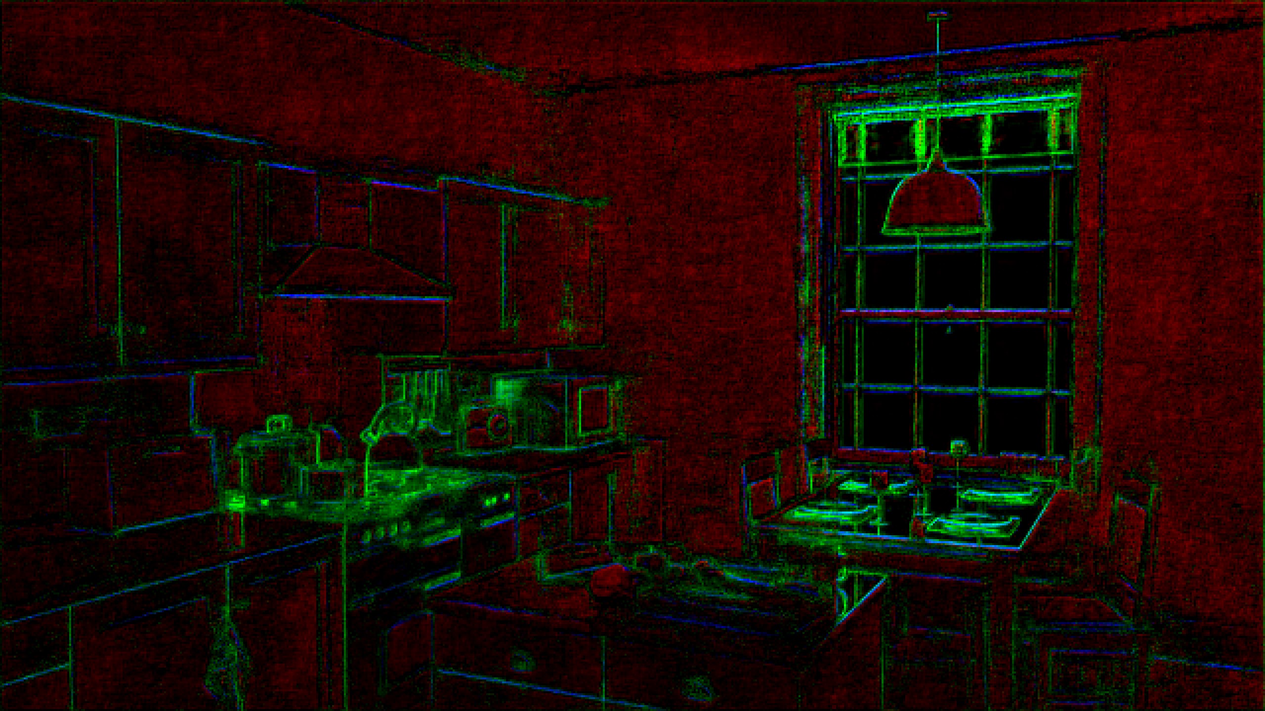
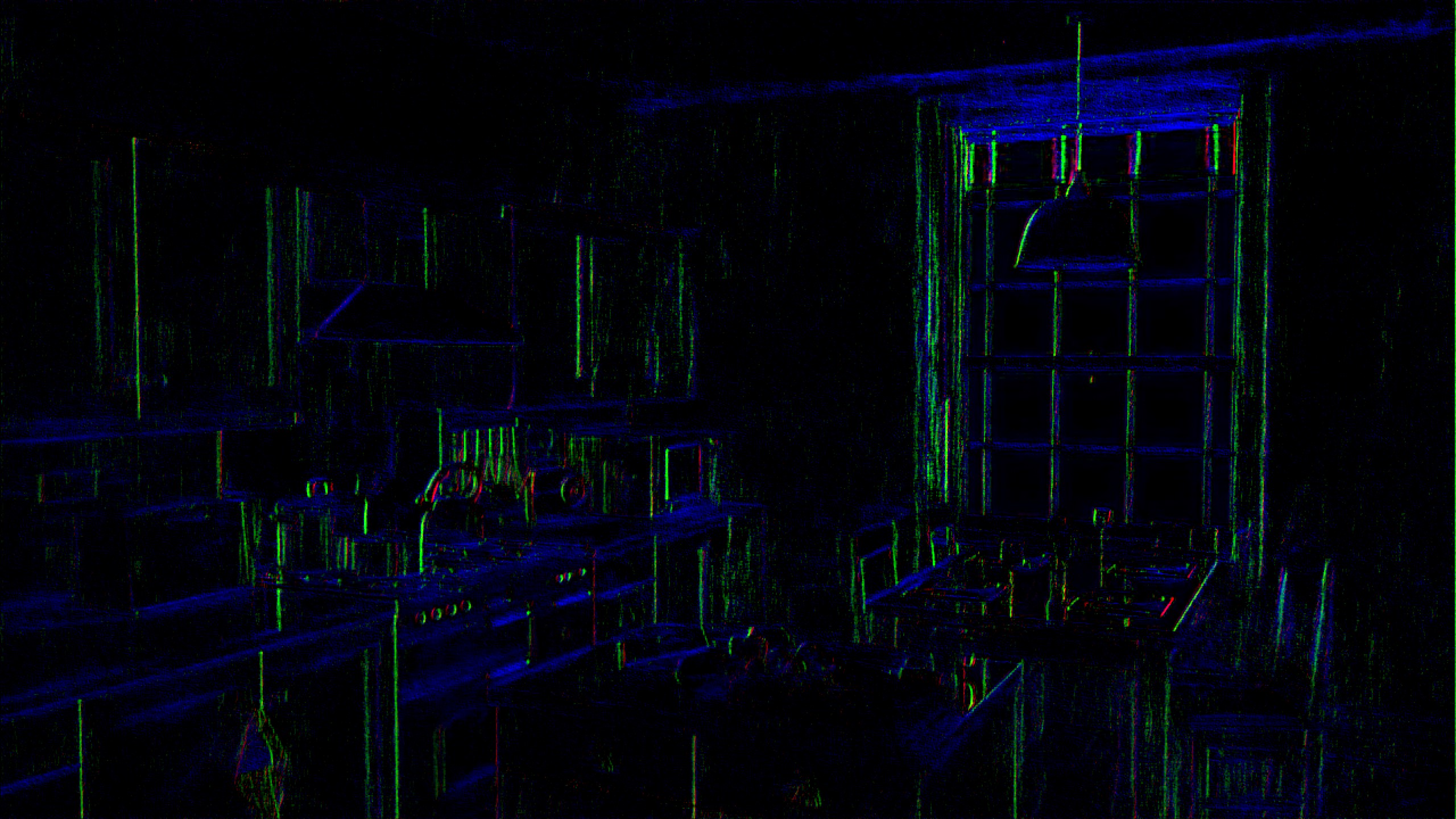
Gallery containing the the output of each pass along with it’s corresponding resoution and channel count.
It’s worth briefly clicking through the gallery above just to get a sense of what’s going on. I can only show 3 channels at a time so this is not an exhaustive visual of the whole operation. Also this only shows the outputs of convolution passes, I’ll break it down later but the outputs of a pooling/upsampling/join pass aren’t visually interesting so I’ve skipped those.
A couple of observations we can make just going through all the passes:
- Resolution starts at 2560x1440 but by the time we get to convolution 7, it’s dropped all the way to 160x90 (1/16th the resolution of our input resolution)!
- Starting from convolution 9, you’ll see that the resolution progressively works it’s way up doubling it’s way back up until it hits 2560x1440
- On the flip-side however, as resolution drops, the channel count skyrockets all the way to 112 channels! And as resolution increases, the channel count continues to drop down.
Operators
Okay lets go through the operators now
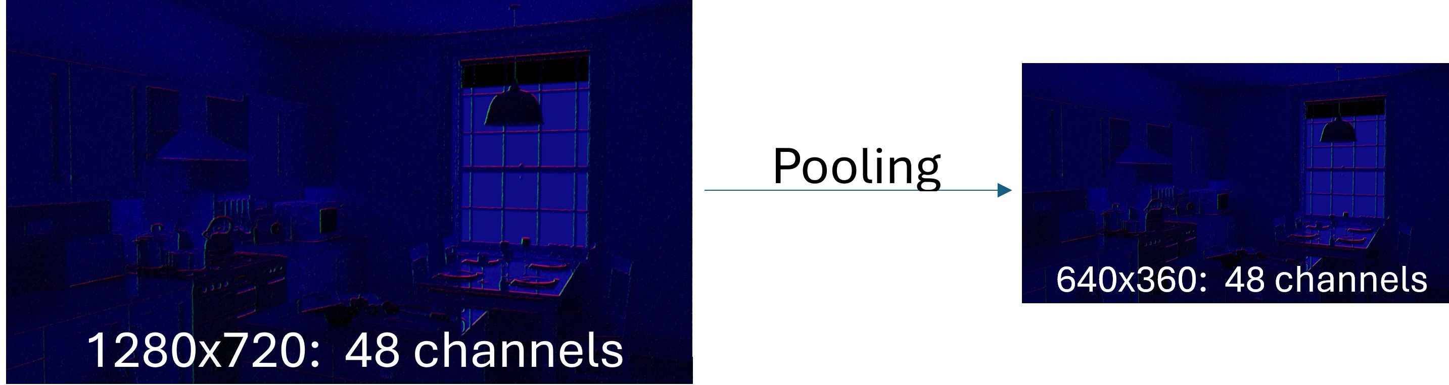
Pooling
This one is easy, it’s simply a downsample. If downsampling to half resolution, this will need to take 4 pixels and combine them into a single pixel. Normally in rendering you would take the average of the 4 but Open Image Denoise chooses to take the channel with the highest value (i.e. just the max).
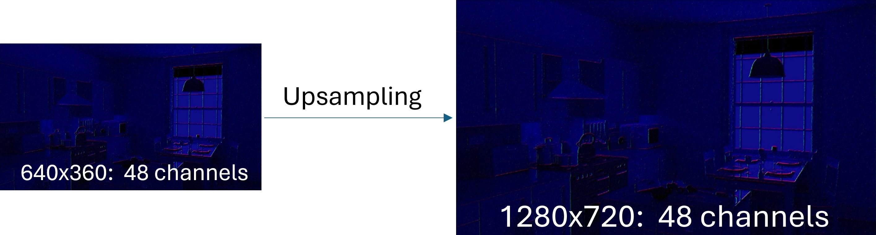
Upsample
This simply upscales the image using nearest neighbor sampling (i.e. not even bilinear!). In OIDN this just doubles the resolution. I’ll say it again, this uses nearest neighbor so the upsample when taken by itself visually will look quite poor, don’t be fooled into thinking there’s magic here! Easy enough I think, lets move on.
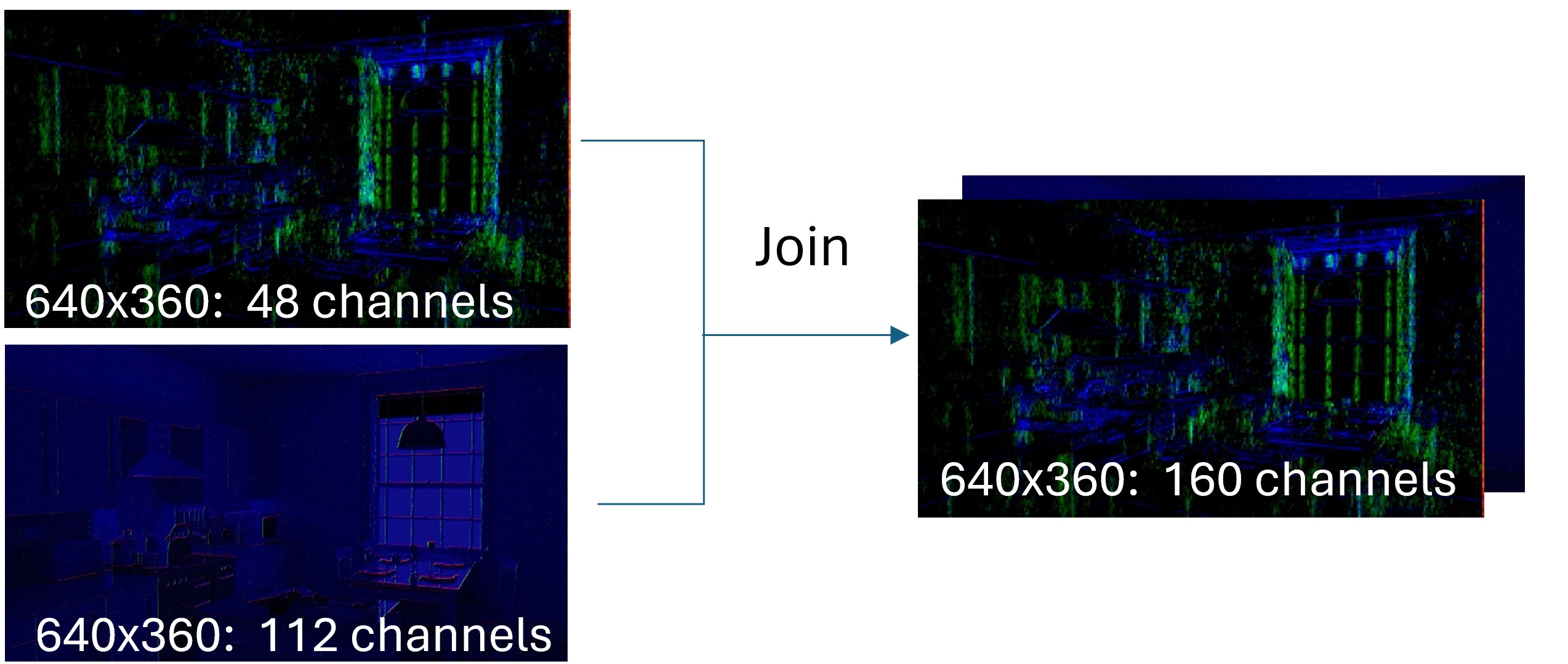
Join
This appends the channels from one tensor to another tensor. So if we have a tensor with 3 channels and another tensor with 6 channels, the resulting tensor would have 9 channels. Some things may also call this a concatenation.
Convolution
Okay the final and most important piece we need to understand. If we go back and look at the frame times of OIDN, Convolution essentially dominates the GPU usage. Luckily, the idea behind convolutions is fairly simple.
A convolution operator takes a filter matrix and applies it to all neighboring pixels. In the context of Open Image Denoise, the filter is always a 3D Matrix. In terms of width and height, all convolution operations (except the last one) are 3x3 and the depth is the number of channels in the input tensor.
Lets take a look at a concrete example. Lets say you want to extract if there’s a vertical edge in the image. The standard way to do this is with a Sobel filter. Here’s the Sobel matrix:
-1, 0, 1
-2, 0, 2
-1, 0, 1
The way this works is fairly straight-forward. At a high-level, you look at your pixel to the left and your pixel to the right. If they’re roughly the same value, they’ll cancel out and you’ll get a value close to 0. If they’re different, you’ll get something non-zero. The further apart they are, the larger the magnitude. We also account for diagonals but they’re weighted slightly less.
However, our input is RGB, so we have 3 channels as input! So what we want is not just a 3x3 matrix, but a 3x3 matrix per channel, i.e. 3x3x3 matrix. Lets say we want to weight the channels so that it takes human perception into account (i.e. the eye tends to be more sensitive to green than blue). The usual weighting looks something like this:
0.3, 0.59, 0.11
We can combine those weights with our Sobel matrix to get our 3x3x3 matrix that we’ll use for our convolution to determine a vertical edge:
-0.3, 0, 0.3        -0.59, 0, 0.59      -0.11, 0, 0.11
-0.6, 0, 0.6        -1.18, 0, 1.18      -0.22, 0, 0.22
-0.3, 0, 0.3        -0.59, 0, 0.59      -0.11, 0, 0.11
Just this simple filter gets us something like this:
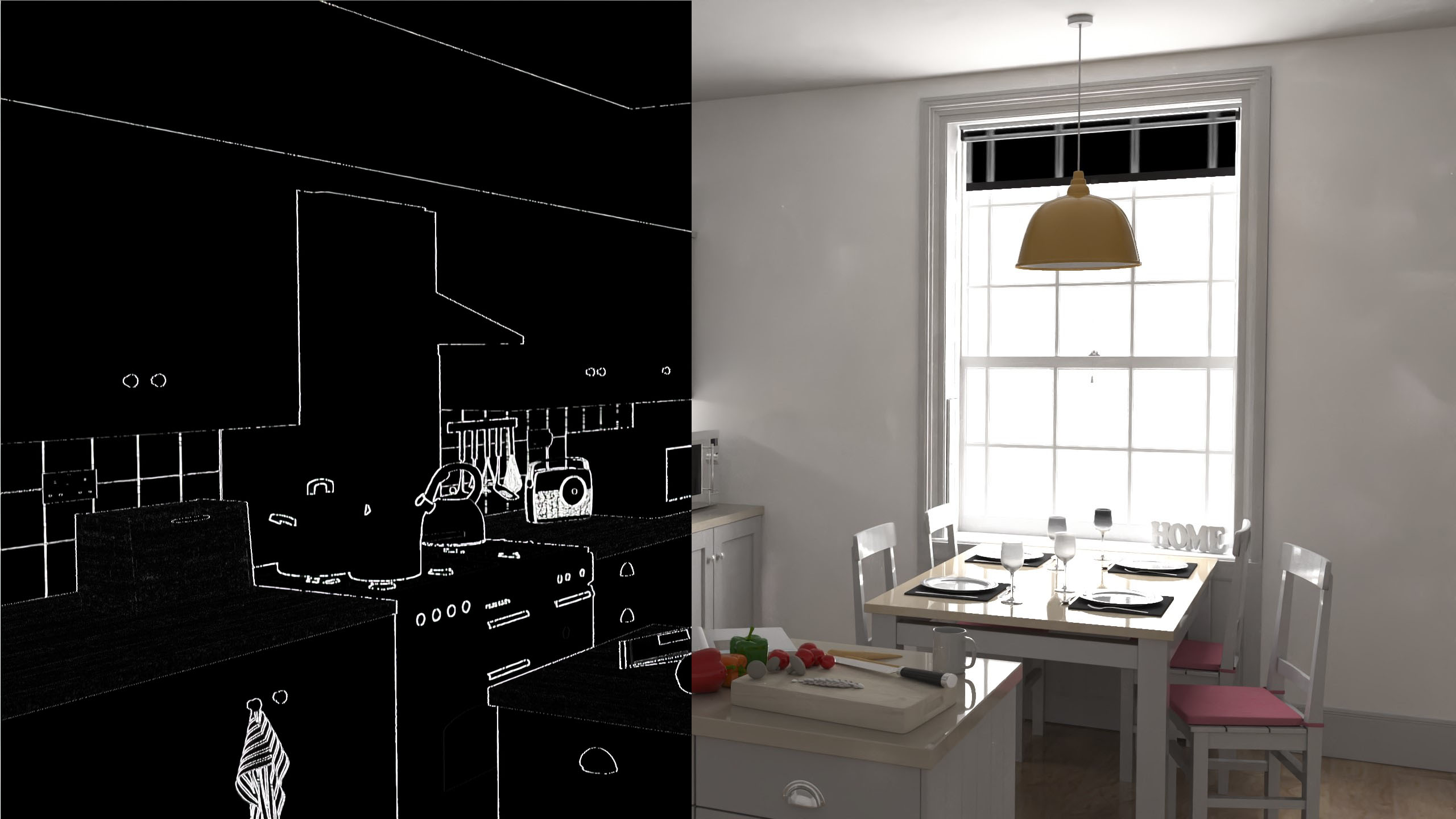
Outlines on the left and input image on the left
Okay great, we’ve got a convolution matrix that can now output one feature! However maybe we want to output another feature…like say, a horizontal edge? Convolution filters allow you to have a list of these 3x3x3 matrices, each one adding a whole new channel to your output. Maybe you also want a filter that detects if the pixel is orange-ish, or if the pixel is a bit blurry. Each of these is an extra 3x3x3 matrix.
Now keep in mind, we’re currently focusing on this very simple case with 3 channels. If your input is 112 channels, then you need a 112x3x3 matrix for each output feature.
Okay that’s all there is to convolution! You now know all there is to know about a single convolution operation in isolation. This by itself might not seem very powerful. However this is where the “deep” part of convolution neural nets come in. We have many, many layers of these convolution operations, each one building on the previous layer. So we were looking at a simple convolution layer that takes in RGB. However the next layer would be taking in inputs like “Is a verticle edge” or “Is horizontal edge”. The next layer you can imagine starts to get more vague like “Has lots of edges” or “Is blurry”. And it gets more and more abstract as OIDN goes down 6 layers of convolution. It’s hard to say what things “mean” at the bottom of the net, but I’d have to imagine it gets to things like “Is skin” or “Is Caustics-ish”.
It’s fairly easy to imagine how this plays well to a GPU’s strengths. You’re doing 3x3 filter * n pixels * m channels * k filters. If we look at the most expensive convolution operation: dec_conv2b, we’re doing 64 filters on a 1280x720 texture with 64 channels: so 3.8 billion 3x3 filters (or 33 billion multiplies).
So who writes these filters? Well, remember those “weights” I talked about when I briefly talked about “learning”. You can start to imagine how that fits in. Machine learning engineers create the arrangement of ML passes and the amount of outputs from each pass, and then a learning pass keeps trying random filters and outputting a final image that gets scored on how well it looks to a golden reference (for path tracing this is easy because we can generate the golden reference by using a very large SPP). There’s a ton of really interesting linear algebra you can use to make sure the learning process is more efficient than just trying random filters, but suffice to say that’s out of the scope of this post.
Putting it all together
Okay we have now covered all the building blocks. What I’ve covered is exhaustively all the operations that run on the GPU when running OIDN. This may surprise you as none of these operations in isolation seems to be enough to be able to denoise the scenarios to the degree that OIDN manages to handle. Especially if you’ve ever written a TAA or denoiser before, that code tends to be filled with tons of special case handling (responsive masks, anti-ghosting, etc). In this case however, all we’re doing is a bunch of convolution filters over and over mixed in with a few downscales and upscales.
I’ve clumsily graphed out a big picture graph of how all these operators come together:
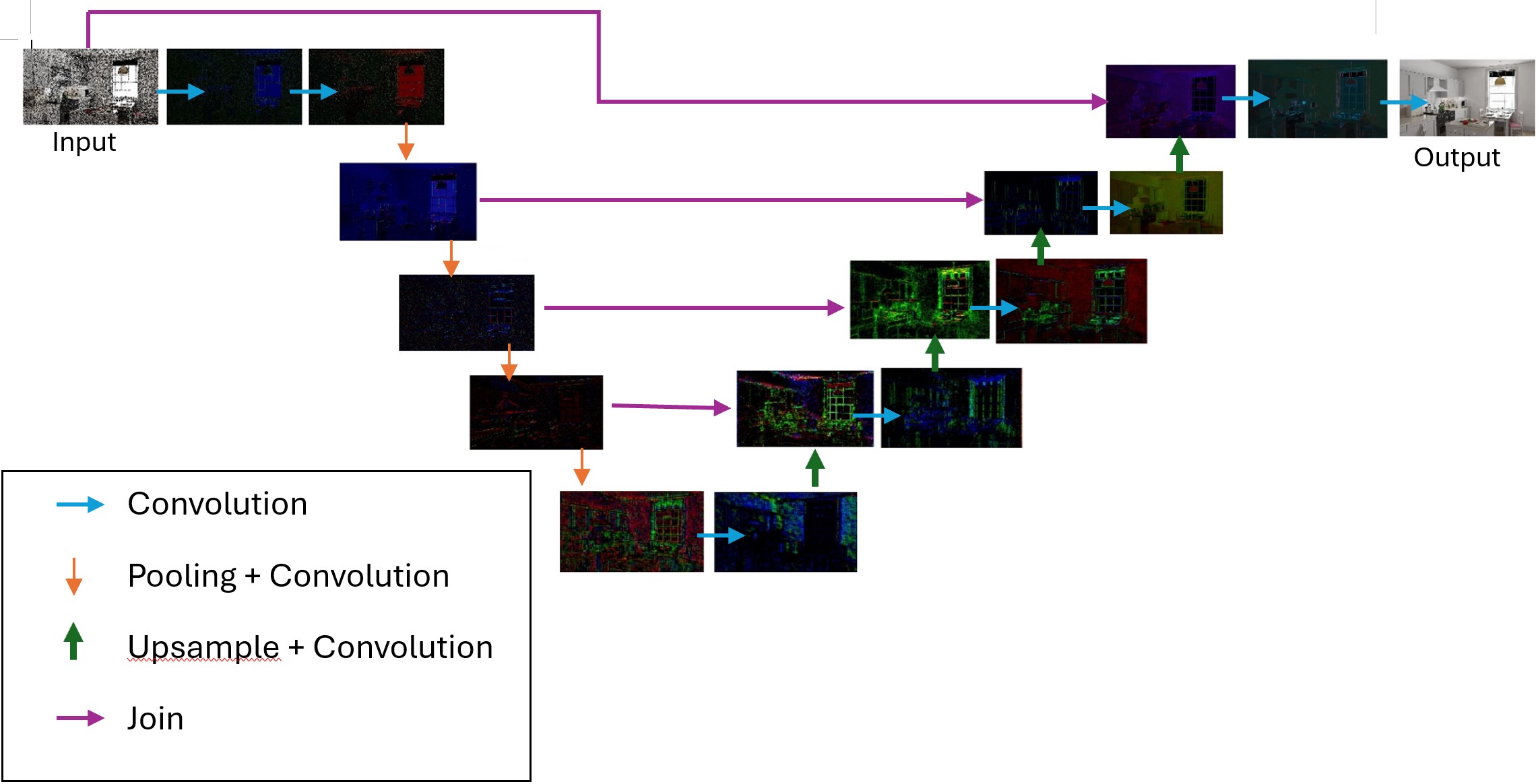
You’ll notice that the flow forms a U-shape. This is because OIDN is based on the concept of a U-Net, which by-and-large means that we can think of the ML execution in 2 steps: an encoding phase and a decoding phase.
In the encoding phase, which is represented in the first left half of the OIDN graph, we reduce the resolution in multiple steps while encoding more and more abstract data into deeper channels. This is done by a series of convolution operators followed by downsample operators. At each convolution operator we are generating more and more channels (i.e. each convolution operator has an increasing amount of filters). By the time we get to the bottom, we’re at 1/16th resolution with 112 channels
In the decoding phase we do the opposite. Essentially we are decoding these “deep” layers of information layer while slowly increasing the resolution via upsample operators until we’re back at the resolution we started with. Each convolution has fewer and fewer filters causing each convolution to output a reduced set of channels until we’re finally back down to our 3 channels (RGB). Notice that each time we increase resolution, we also tack on information from an earlier step via a join operator. This is an important step to note because recall that we dropped all the way to 1/16th res at the end of the encoding step. Recall the upsamples are just naive nearest neightbor upsamples, if we just did that all the way back to full resolution, you’d get a blurry mess. However by using the join, we get information that’s still twice the resolution of the thing we just upsampled. The following convolution can then combine the 2 and intelligently upsample based on the vast channels of information. I say “intelligently upsample”, but on the GPU it’s just a ton of multiplies, the smart logic is all coming from the weighting that came from the learning process.
Conclusion
Okay that’s a wrap. If you were hoping to become a machine learning expert after reading this, uh…this is not the post you were looking for. But hopefully if you came from having no idea what machine learning is, you now have some sense of what’s running on your GPU and what the work is involved. I narrowed in on a small slice of machine learning workloads: Convolution Neural Nets. There’s so much more to machine learning so this is just a small case study. If you’re like me, I learn best from this kind of depth-first approach, in contrast to breadth-first which in machine learning is insanely broad.
If you want to learn more about machine learning in a broad sense, here’s a few resources I’ve found extrememly helpful:
- Max Liani’s Deep Neural Network Dive posts - These are so, so very good. As I mentioned, my post is basically a rehash of his but just from a different perspective. I would go as far as saying I could not have accomplished my DirectML port without these posts. What I love about his posts is Max is a rendering engineer and so it’s explained from the perspective of a machine-learning “outsider’ which I think helps him explain things in a way that reads very naturally for us average Joes. If you just read one of my resources, read this one.
- Neural Networks and Deep Learning - This is essentially a textbook that’s freely available online. I’ll admit I haven’t read the whole thing and I didn’t do any of the exercises. But when I was starting to wrap my head around what is machine learning, this is was the best resource to breaking down the low level building blocks. If you’re interested Things like operators, weights, biases, etc, I would absolutely recommend this as a starting resource.
- SIGGRAPH: Hands-on Workshop: Machine Learning and Neural Network: Similar to the above, I’ll admit I didn’t do the exercises. But this was an interesting overview that focused more on the high level details of a neural network